Stefan Zellmann's Blog – Stefan Zellmann's Blog — Here I blog about my research on (mostly…) parallel graphics and visualization.

Exajet, a huge time-varying AMR simulation data set comprised of >400 time steps, each clocking in at 4×2.5 GB of scalar data. Data courtesy Pat Moran and available online here: https://data.nas.nasa.gov/exajet/.

This week I gave a talk for our “AMR Streaming” paper [1], with Ingo Wald, Alper Sahistan, Matthias Hellmann, and Will Usher. The paper is a follow-up to our original paper [2] at VIS in 2020 and “simply” adds support for time-varying data with SSD to GPU streaming updates to our ExaBricks software.

The central figure of this paper at first sight looks innocent enough, but when taking a closer look contains so much detail, trial and error, completely back to the drawing board phases that a simple paper and talk at a symposium just don’t do it justice.

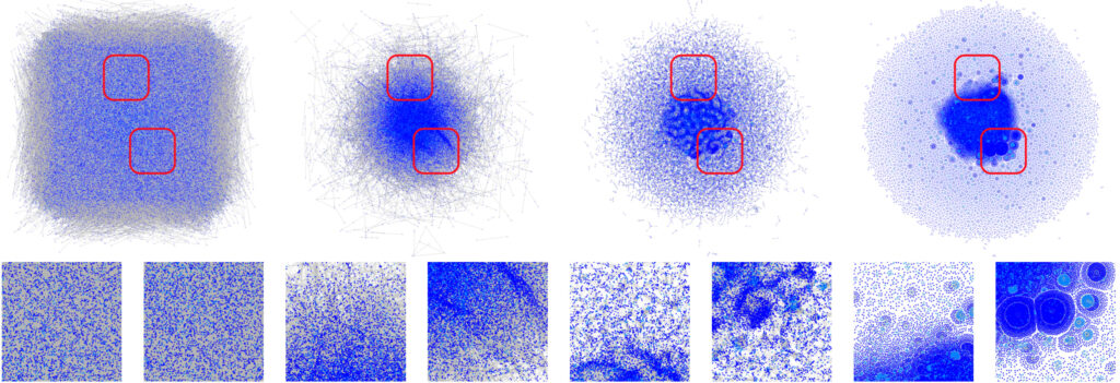
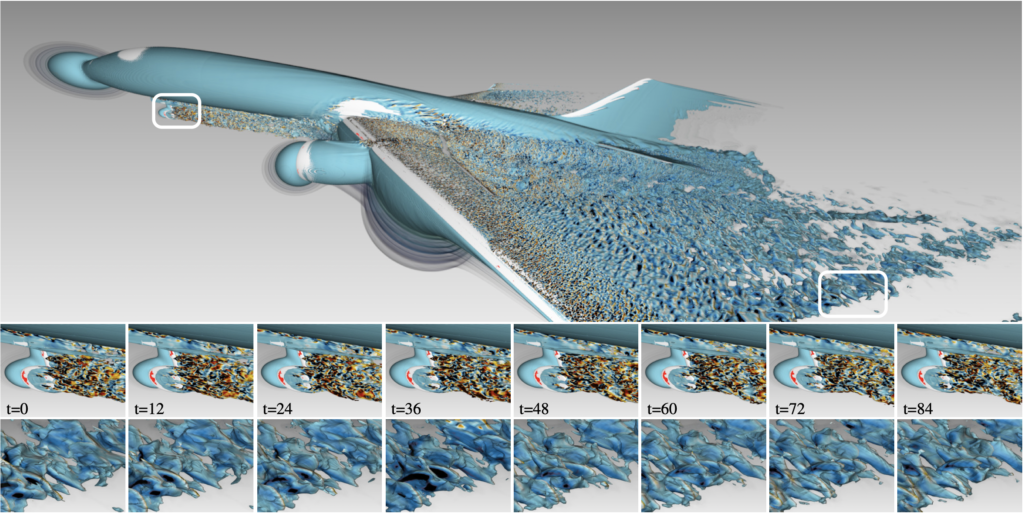
Here’s that central figure:

Figure 3 from our paper, with all the gory details how we eventually ended up implementing streaming updates in our ExaBricks software

What the paper does is take our original ExaBricks software, pick a couple of representative snapshots of NASAs exajet, and extend the software to support fast streaming updates, as the data set as a whole is huge: 400 time steps at roughly 10 GB (4 fields with 2.5 GB each).

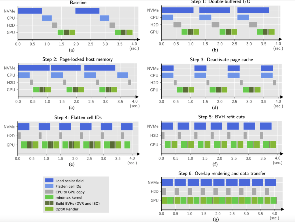
Now Fig. 3 from the paper presents a couple fairly straightforward optimizations; adding double buffering to overlap file I/O with compute. Using pinned memory to achieve faster copy performance from host to device; unrolling cell ID indices that map 1:1 into scalar fields; deactivating the OS page cache to reach maximum SSD/NVMe read bandwidth, etc etc. The list is long and the measures we have taken compound, yet from a scientific perspective, they’re admittedly simple if not trivial: one might even argue they’re “obvious”. There’s a small number of algorithmic improvements we propose, but still.

But recalling how that paper and software actually came to be, reminds me that the process was anything but simple or trivial, let alone obvious. If you take a look at Fig. 3 above, you can see how the first illustration shows what happens if you simply take ExaBricks and exajet, and just run the software on each individual time step. The result is a two seconds round trip per frame rendered, including the file I/O, GPU copies, and general data wrangling that are necessary to render these frames. The transformations we applied to this naïve baseline gradually squeeze the individual processes, shave off a couple milliseconds here and there, make some improvements to build BVHs more efficiently, to finally arrive at a design that is more or less general and streamlined for high-quality rendering of very large, time-varying AMR data.

Now here’s what the figure does not show: the original design we came up with (and actually fully implemented…) was totally different; see how the final design in Fig. 3 is static: we use double-buffering, could potentially also squeeze things more and eventually move to a design that does triple buffering; but the original design we had was a dynamic LRU cache implemented with a host-side queue that could accommodate N (on the order of 30 or 50) time steps, and was filled in a background thread, and another, much smaller queue for host-to-device transfers. That system was functional (and there was actually quite a bit of engineering effort and technical debt that went in there), but eventually proved to be ineffective. The LRU cache was generally hard to maintain as a piece of software; but most problematic was unpredictable performance behavior when a time step was dynamically loaded and we were at the same time copying data to the GPU.

We struggled a while with this design, but eventually gave up on it, although in our mind it was the “obvious” thing to do (that’s actually reflected in the literature, and there was even another AMR streaming paper [3] at EGPGV that focuses on CPU rendering and that does use this type of design); but with the two devices connected over PCIe 4.0 (SSD and GPU) just would not scale (for us; in practice..). So, back to the drawing board, throwing all the stuff we had so far over board and redesigning the system from scratch.

File I/O… you might think, that when using a fast NVMe SSD, you’d just use the usual fopen/fread machinery (and avoid C++ streams), and then the copies be as fast as it gets. Turns out that.. no, as the operating system’s page cache is getting in your way; performing a literature study on low-latency file I/O, you’ll find there’s a whole research area looking into and optimizing what’s basically nothing else but fast reads from SSDs (what we finally ended up doing was deactivating the page cache altogether using system calls, this also turned out to give more consistent results, and we were already planning to do this anyway to give more consistent benchmark results as well).

Question from the audience: “did you guys consider using managed instead of host-pinned memory?!”… well, sure. We did. Turned out to be 1.5 to 2x slower; so, here goes another round of experiments.

And there’s a whole list, these are just the tip of the iceberg. With the exception of our takes on page caches and read operations, non of this actually made it into the final paper; that just contains that innocent looking list with simple (if not trivial) optimizations that eventually gave us a speedup of 4x over the baseline.

Then, there’s a limitation, in that AMR hierarchies often change with time, but ours aren’t allowed to (exajet does not); so obviously, we were called out by the reviewers for not mentioning this prominently enough, and sparked a bit of discussion (also thanks to Pat Moran who published the exajet data set for providing some valuable insights there) as of how realistic that property of the data actually is. In aeronautics, it’s actually not uncommon that engineers/scientists know in advance what good seed regions are, and then place their seeds there and fix the hierarchy over time, because the macro structure is just known a priori (and safes them both simulation time and memory).

From our side, for now only supporting this kind of data is of course a limitation (and points to some obvious… yet not trivial future work). But with a different group of reviewers, could definitely have ended differently, if not with the paper bouncing.

In summary, it’s just fascinating how much work can go into a single paper, and how compressed the final information becomes on these 8-9 pages, given all the hoops you have to jump through to finally arrive at the results that make it into the paper. That said, we hope that the lessons we learned from the process also help others with their decisions and they’ll apply them to their own large data and GPU related problems. And if you haven’t done so, go ahead and read the paper; an authors’ copy can be found here.

[1] S. Zellmann, I. Wald, A. Sahistan, M. Hellmann, W. Usher (2022): Design and Evaluation of a GPU Streaming Framework for Visualizing Time-Varying AMR Data. EGPGV 2022.

[2] I. Wald, S. Zellmann, W. Usher, N. Morrical, U. Lang, V. Pascucci (2020): Ray Tracing Structured AMR Data Using ExaBricks. IEEE VIS 2020.

[3] Q. Wu, M. Doyle, K.-L. Ma (2022): A Flexible Data Streaming Design for Interactive Visualization of Large-Scale Volume Data. EGPGV 2022.

That’s my first post on this blog, and as such–in regards to the blog’s title–it actually falls into the “mostly…” category. It’s about a short paper we recently got accepted at IEEE Visualization with Martin Weier and Ingo Wald and is called Accelerating Force-Directed Graph Drawing with RT Cores.

Here’s a link to that paper on researchgate: https://www.researchgate.net/publication/343904020_Accelerating_Force-Directed_Graph_Drawing_with_RT_Cores

The idea is to use NVIDIA’s RTX ray tracing extensions for something other than graphics and rendering and is motivated by this paper where the authors used RTX to accelerate point-in-tet queries.

In this paper, we use RTX to accelerate force-directed graph drawing, which is concerned with finding nice layouts for (usually 2D) graphs; nice means–amongst others–that there aren’t too many edge crossings and generally that vertices that are connected by edges are relatively close-by. The most simple force-directed algorithms treat the graph vertices as particles, with mutual forces acting on each particle and the overall, physically inspired system trying to reach equilibrium w.r.t. those forces.

At the heart of the force-directed algorithm is a nearest-neighbor query where we find–for each vertex/particle in parallel–all the neighbors within a certain radius, and then compute repulsive forces from them.

For example, in the image above, the two green vertices inside the large circle act forces upon the red vertex, and in order to find those vertices, we just expand a circle of radius k around the red vertex to gather all its neighbors. This type of nearest neighbor query can be easily implemented with a quadtree or a kd-tree over the particles that we traverse by only considering the inner nodes, and later the leaf nodes and particles that are within the large circle.

As it just so happens, for the force model that we chose, this large circle’s radius k is always the same, and this allows us to reverse that algorithm. Instead of building a hierarchy over particles, we instead build a bounding volume hierarchy over circles:

The circles have their centers at the vertex/particle positions, and the radius is the same as the search radius we used for the nearest neighbor query from before.

Now, instead of using a nearest neighbor point query–in software and therefore slow, also laborious to code up the kd-tree construction and traversal code–we can just shoot a ray through the bounding volume hierarchy (and obviously, that’s what we use RTX for).

It doesn’t matter in which direction the ray is pointing and we therefore choose an arbitrary vector with infinitesimal length to keep the number of BVH node tests minimal. It’s only important that the ray’s origin is located at the vertex position that we’re interested in:

The circles that overlap the ray origin belong to the particles that act forces on the vertex of interest (we’ll also hit the circle of the very particle that we’re testing for–here in gray–but just ignore that during traversal).

It turns out that this is really easy to implement with OptiX and RTX. We just build a user geometry over the circles and a BVH, and in the intersect program we check if the circles that we’re presented with overlap the query ray. If so, we’re in the range where mutual forces are active; in fact, this query will give us the exact same particles that we would have gathered using the NN query. Using RTX for this is actually quite fast, we beat a fairly optimized, hand-tuned CUDA LBVH implementation by several integer factors.

A limitation is that the force model we’re using is a bit outdated–yet very simple to implement-and as such, our study is a proof of concept; we’re already working on other force models like FMM that will converge faster than the simple model we used in the paper and we’re confident that we’ll also see decent speedups for those.

Obviously, all that works because the radius is the same, no matter which particle we’re evaluating forces for. That restriction is actually not so bad; most graph networks have weights associated with the edges, but not with the vertices. As such, vertices have no area (volume in 3D), and thus we can just assume that for our physical model the particles have no mass. It would of course be interesting to implement that approach for particles having a mass, but then we wouldn’t get away with such an easy query.

The paper will be presented at this year’s IEEE VIS (due to the pandemic they will stream the talks online and attendance is free). Sample code for the paper can be found on github: https://github.com/owl-project/owl-graph-drawing

Although the idea is relatively simple, it shows a nice way to use the NVIDIA RTX hardware extension for sth. completely different than rendering; I’m excited to see what the future brings on this front and what clever ideas people will come up with for that they can use ray tracing in a similar fashion, and I hope that this paper is a little inspiration for them!